
Multi-agent gridworlds
Gridworlds are popular environments for RL experiments. Agents in gridworlds can move between adjacent tiles in a rectangular grid, and are typically trained to pursue rewards solving simple puzzles in the grid. MiniGrid is a popular and flexible gridworld implementation that has been used in more than 20 publications.
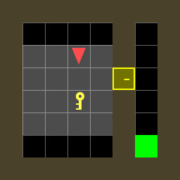
I’ve created a multi-agent variant of MiniGrid called MarlGrid. In the modified library, multiple agents exist in a shared same environment: they can observe each other and aren’t allowed to collide. At each time step, the agents view distinct portions of the environment, act independently, and receive separate rewards. Scenarios can be a mix of competitive and collaborative, depending on the structure of the reward signals. MarlGrid could be valuable to other multi-agent researchers, so feedback and contributions are welcome!
DQN
While working on the multi-agent environment, I’ve been using deep Q learning to train independent agents to accomplish the simple task described above. The agents’ behavior is guided by separate deep Q networks (DQN) that predict the best action to take based on their observations. This technique, sometimes called Independent Q Networks or IQN, can effectively train agents in very simple scenarios:
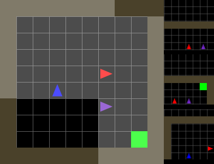
But IQN has shortcomings that manifest in larger or more complex environments.
Below, I’ll review DQN and explain some of these issues.
Deep Q-learning review
In Q learning, the behavior of the agent is determined by a Q function $Q(s, a)$ that estimates the value of a state $s$ conditional on taking a particular action $a$. The value of a state (at time $t$) is taken to be the expected $\gamma$-discounted sum the of the rewards $r_{t^{‘} \geq t}$ the agent would subsequently receive. The procedure by which an agent chooses an action based on the state is known as the agent’s policy $\pi$. When the environment is in state $s_{t}$, the agent takes the action $a_{t}$ that maximizes $Q$:
\[a_{t} = \pi(s_{t}) = \underset{a}{\text{arg}\,\text{max}}\ Q(s_{t}, a) \label{eq:qpolicy}\]Classical Q learning assumes the set of possible states $S: s_{i} \in S$ and possible actions $A: a_{j} \in A$ are both finite. Then the Q function can be represented by a table where the value in cell $(i,j)$ is $Q(s_{i}, a_{j})$, i.e. the expected value of taking action $a_{j}$ in state $s_{i}$. A variant of this technique called deep Q learning also applies to continuous state spaces, using a neural network (DQN) approximation rather than a tabular representation of the state-action value function $Q$. DQN was developed by Mnih et al (2013) and achieved impressive results on a suite of Atari games.
This value estimation problem is central to reinforcement learning: rather than predicting the immediate rewards the agent might receive by taking a greedy action now, the goal is to estimate all of the future rewards it can attain starting from this state. This is why reinforcement learning is sometimes referred to as sequential decision making.
In Q learning, experience collected by an agent (behaving per $\text{eq.}~\ref{eq:qpolicy}$) is used to update $Q$ with a method called value iteration, which seeks to minimize the loss:
\[L = \left\lVert Q(s_t,a_t) - \left( r_t + \gamma\ \underset{a}{\text{max}}\ Q(s_{t+1}, a) \right) \right\rVert\]Iteratively minimizing this loss leads to continual improvements in the Q function when the environment in which the agent is situated can be described by a stochastic Markov decision process (MDP) (Jaakkola et al 1994). An MDP is characterized by $(S, A, T, R)$, where $S$ is the set of possible environment states, $A$ is the set of possible actions, $T:S \times A \rightarrow S$ is the transition function, and $R:S\times A \rightarrow \mathbb{R}$ is the reward function. For an environment to be an MDP, $T$ and $R$ must be stationary: the reward $r_{t}$ and new state $s_{t+1}$ resulting from the agent taking an action $a_{t}$ in a state $s_{t}$ can’t depend on any states or actions from before $t$ (Markov assumption).
Challenges in multi-agent training
In IQN, value iteration is used to simultaneously and independently train multiple DQN agents. The environment overall can still be described as an MDP, but the states and rewards observed by the individual agents no longer obey the Markov assumption: individual agents don’t control all the actions that determine the transition of the global environment state, and may only have partial views of that state (as in the MarlGrid examples).
Non-stationarity
In a $k$-agent gridworld, the transition function depends on the actions of all the agents: $ s_{t+1} = T(s_{t}, a_{t}) = T(s_{t}, a_{t}^{1}, a_{t}^{2}, …, a_{t}^{k})$. So from the perspective of a agent $i$, the transition depends not only on the state and its action $a_{t}^{i} = \pi^{i}(s_{t})$, but also on the actions $\{ a_{t}^{j} = \pi^{j}(s_{t}), j \neq i \}$ of the other agents.
If the policies of the other agents were static, then their actions could be seen as aspects of the environment state invisible to the $i$-th agent, and this would boil down to an issue of partial observability. But since the policies change as the agents learn, $T$ is non-stationary from the perspective of any single agent.
Partial observability
Individual agents in the MarlGrid environments have limited fields of view. Even in relatively simple environments, this limits the sophistication of agent behavior.
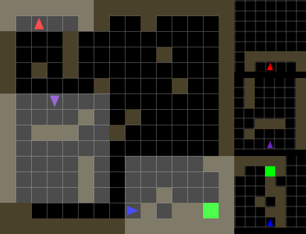
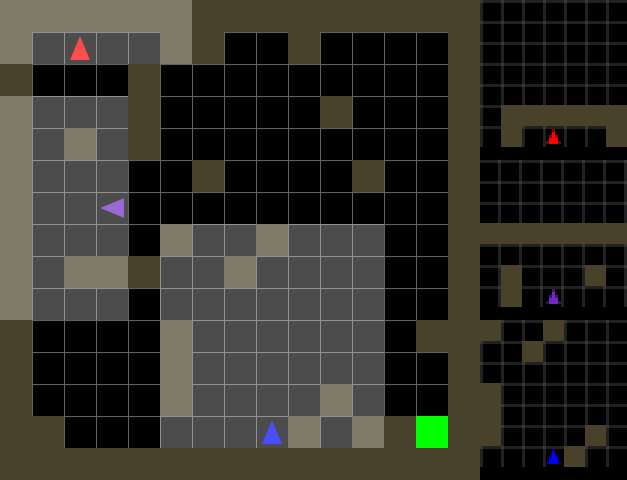
Right: Having rotated, the blue agent can no longer observe the goal. Since the agent's policy can only generate actions based on the current observation, the agent is unlikely to follow a sequence of actions that will lead it to the goal.
As another example, the purple agent in the second video above ends up spending lots of time wandering aimlessly. Since the agent lacks memory, it is unable to develop a strategy that would help it systematically explore the environment.
This shortcoming of basic DQN implementations is typically mitigated by giving the agent some capacity to account for observations prior to $s_t$ when determining an action $a_t$. The Atari DQN collaboration (Mnih et al 2013) accomplished this by giving agents direct access to some of 16 previous frames. Hausknecht et al (2015) addressed this using deep recurrent Q networks (DRQNs) that use RNNs to explicitly maintain state across multiple steps in the environment. I plan to take the latter approach. Next week, I will incorporate LSTM cells into my DQN in order to give agent’s memory, and improve their ability to handle partial observability and model other agent’s behavior.
References
Volodymyr Mnih et al. Playing Atari with Deep Reinforcement Learning. arXiv preprint arXiv:1312.5602, 2013.
Tommi Jaakkola et al. On the convergence of stochastic iterative dynamic programming algorithms. Neural Computation, 6 (6): 1185-1201, 1994.
Matthew Hausknecht et al. Deep Recurrent Q-Learning for Partially Observable MDPs. arXiv preprint arXiv:1507.06527, 2015.