
DQN and DRQN in partially observable gridworlds
RL agents whose policies use only feedforward neural networks have a limited capacity to accomplish tasks in partially observable environments. For such tasks, an agent may need to account for past observations or previous actions to implement a successful strategy.
As I mentioned in a previous post, DQN agents struggle to accomplish simple navigation tasks in partially observed gridworld environments when they have no memory of past observations. Multi-agent environments are inherently partially observed; while agents can observe each other, they can’t directly observe the actions (or history of actions) taken by other agents. Knowing this action history makes it easier to predict the other agent’s next action and therefore the next state, leading to a big advantage for agents that have some form of memory.
One way to address the issue of partial visibility is to use policies that incorporate recurrent neural networks (RNNs). In this post I’ll focus on deep recurrent Q-networks (DRQN, Hausknecht et al. 2015) in single-agent environments. DRQN is very similar to DQN, though the procedure for training RNN-based Q-networks adds some complexity.
In particular, I’ll discuss
- differences between DQN and DRQN,
- ways to manage the hidden state for recurrent Q-networks, and
- empirical advantages of DRQN over DQN
DQN
The key component of DQN is a neural network that estimates state-action values $Q(s_{t}, a_{t})$ – the values of states $s_{t+1}$ induced by taking any possible action $a_{t}$ in a given state $s_{t}$. In DQN (and DRQN) we assume the action space is discrete, i.e. $a^{0} = \text{move forward, } a^{1} =\text{rotate left, }$etc, and for the examples in this post the “states” observed by the agents are images.
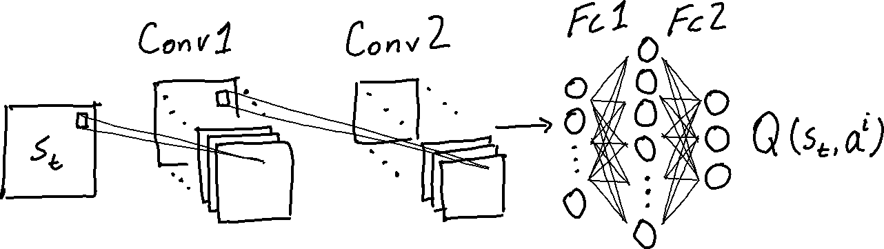
When presented with a new environment state $s$, the agent estimates the state-action values $Q(s, a’)$ of all possible actions $a’$ then selects the action with this highest value, e.g. $a = \pi(s) = \text{arg max}_{a’} Q(s, a’)$. During each episode the agent records the sequence of states/actions/rewards. Between action steps the agent uses value iteration to update the weights of its Q-network, minimizing
\[\text{Loss}(\theta) \dot{=} \left\lVert Q^{\theta}(s_t,a_t) - \left( r_t + \gamma\ \underset{a}{\text{max}}\ Q^{\theta}(s_{t+1}, a) \right) \right\rVert .\]The agent uses samples of past transitions (stored in a replay buffer) to estimate the loss, and uses some variant of stochastic gradient descent (SGD) to minimize the loss wrt. the network parameters $\theta$.
- loss $\leftarrow$ 0
- Sample a batch of $N$ transitions from the agent's replay buffer
- For each sampled transition $(s, a, r, s')$:
- $v \leftarrow r + \gamma \cdot Q^{\theta}(s, a)$
- $\hat{v} \leftarrow \text{max}_{a'} Q^{\tilde{\theta}} (s', a')$
- loss $\leftarrow$ loss $+ \left\lVert v - \hat{v} \right\rVert$
- Update parameters $\theta$ to minimize loss.
This procedure computes $\hat{v}$ with a target Q-network $Q^{\tilde{\theta}}$. The target Q is a snapshot of the regular Q-network, whose weights $\tilde{\theta}$ are periodically copied from the main Q-network. This helps prevent overestimation of state action values, which is a common issue in DQN.
DRQN
In DRQN some of the post-convolution layers are replaced by an RNN, typically a long short-term memory (LSTM) cell. RNNs are called recurrent because because the output of the cell at one timestep is fed back into itself to compute the output at the next timestep. The “hidden state” $h_{t}$ is a form of memory that gives recurrent cell the capacity to store information between timesteps, and allows them to learn patterns that unfold over time. LSTMs use special gates that control the flow of information into and out of the hidden state, and to forget inconsequential hidden state information. For an excellent overview of RNNs and LSTMs, check out this post on Chris Olah’s blog.
The process by which DRQN agents select actions is the same as in DQN, but the agent uses information from the hidden state in addition to the observed state $s_{t}$ – so the agent needs to keep track of the hidden state over the course of each episode. Typically the hidden state $h_{0}$ is set to zero at the beginning of each episode.
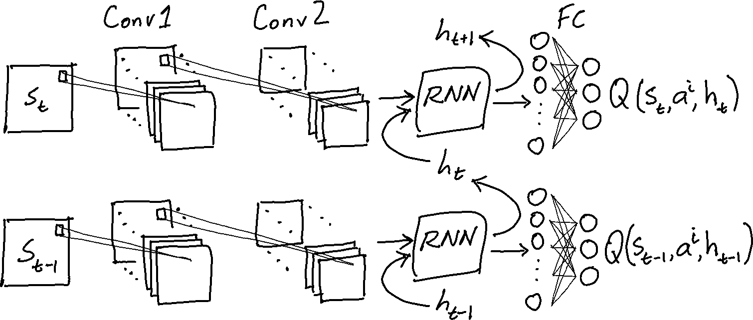
The output of the network at time $t$ depends on the hidden state value $h_{t}$, so it’s instructive to write the Q-function expressed by the network (with weights $\theta$) as $Q^{\theta}(s_{t}, a_{t}, h_{t})$. The network’s RNN layer transforms the hidden state $h_{t} \rightarrow h_{t+1}$; for convenience, we can define a function $Z$ that maps observed states, actions, and hidden states to Q-values and new hidden states: $Z^{\theta}(s_{t}, a_{t}, h_{t}) \dot{=} (Q^{\theta}(s_{t}, a_{t}, h_{t}), h_{t+1})$
The DRQN gradient update similar to the DQN gradient update:
- loss $\leftarrow$ 0
- Sample $N$ replay sequences of length $T+1$ from the agent's replay buffer
- For each sampled sequence $(s_{0 \ldots T}, a_{0 \ldots T}, r_{0 \ldots T})$:
- Initialize hidden state $h_0$
- For $\tau$ in $0 \ldots T-1$:
- $\left( x, h_{\tau+1} \right) \leftarrow Z^{\theta} (s_{\tau}, a_{\tau}, h_{\tau})$
- $v \leftarrow r_{\tau} + \gamma \cdot x$
- $\hat{v} \leftarrow \text{max}_{a'} Q^{\tilde{\theta}} (s_{\tau+1} , a' , h_{\tau + 1})$
- loss $\leftarrow$ loss $+ \left\lVert v - \hat{v} \right\rVert$
- Update parameters $\theta$ to minimize loss.
Keeping track of hidden states
The DRQN update procedure needs some way to $\text{initialize hidden state } h_{0}$ for trajectory sampled while updating the network. Updating the RNN parameters changes the way it interprets hidden states, so the hidden states used originally by the agent to compute its actions aren’t necessarily helpful for later updates.
The original DRQN paper suggests zero-initializing the hidden state at the beginning of each sampled trajectory, but points out that this limits the RNN’s capacity to learn patterns longer than the sampled sequence length $T$.
An alternative approach is to use $Z^{\theta}$ to calculate $h_{t}$ from scratch by evaluating the network for the whole sequence of observations $s_{0} \ldots s_{t-1}$ while keeping track of the hidden states. This can be quite costly since the sampled sequences can occur anywhere in an episode and the episodes can have many more than $T$ steps. For example, if we want to train on a 10-step sequence where $t=990…1000$, we’d need to run the RNN over the first 989 timesteps to get $h_{990}$.
As part of the R2D2 algorithm, Kapturowski et al. (2019) suggest storing hidden states in the replay buffer and periodically refreshing them. When it’s time to update the weights of the policy network, the initial hidden state for each sampled sequence is read directly from the replay buffer alongside the states/actions/rewards. This nominally allows the agent learn to keep useful information in its hidden state through an entire episode, but introduces the potential issue of hidden state staleness: the network parameters might get updated many times before the hidden state is refreshed. Still, Kapturowski et al. show that agents trained with stored/periodically refreshed hidden states outperform those that use zero-initialization in most of the partially observable tasks that they consider. This is the strategy I use in my DRQN implementation for the comparisons that follow.
When the stored hidden states are not stale, refreshing them should only cause small changes to their values. To monitor hidden state staleness, I’ve been logging the cosine similarity between the old and new hidden state values during each refresh (averaged over every episode in the replay buffer).
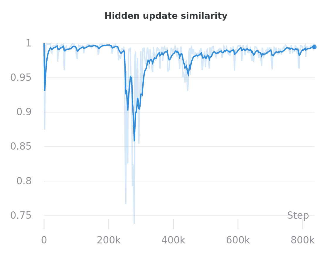
In this example, the agent seems not to make much use of the hidden state until about step 200k. Updates to the LSTM between steps 200K and 400k seem result in relatively volatile changes to the stored hidden states.
DQN v. DRQN in empty gridworlds
Notes/caveats
- In all the environments shown below, agents receive a reward of +1 if they attain the goal state within a time limit, and 0 otherwise. Since the reward signal itself doesn’t distinguish between skilled agents who get to the goal quickly and unskilled agents who meander before stumbling into the goal, the agent skill comparisons that follow use episode length (averaged over 25 episodes, then smoothed) rather than episode reward.
- Vanilla DQN-style $\epsilon$-greedy exploration was very finicky for the DRQN network; using a Boltzmann exploration policy and entropy regularization helped significantly. All of the results shown here (for both DQN and DRQN) incorporate these tricks.
- It was harder to get DRQN working than DQN. The extra effort I put into tuning DRQN might unfairly advantage it in this comparison.
- Thanks to the LSTM, the DRQN networks have more parameters than the DQN networks. Adding more or larger layers to the DQN’s post-convolution MLP didn’t seem to help very much, but I haven’t explored that with much rigor.
- Batch sizes and update frequencies for the two variants were the same, but each element of the DRQN batches were sequences (of length 20 steps) rather than individual transitions so the DRQN updates included contributions from many more individual timesteps.
- All the curves shown here are for single training run (not averaged over multiple seeds).
- The videos I’ve selected are representative of agent performance somewhat late in the training process.
Empty environment
In the “empty” environment variants, agents spawn at a random location and need to navigate to the green goal tile at the bottom right of the grid. In these experiments the grid has size $8\times8$, and the episode time limit is 100 steps.
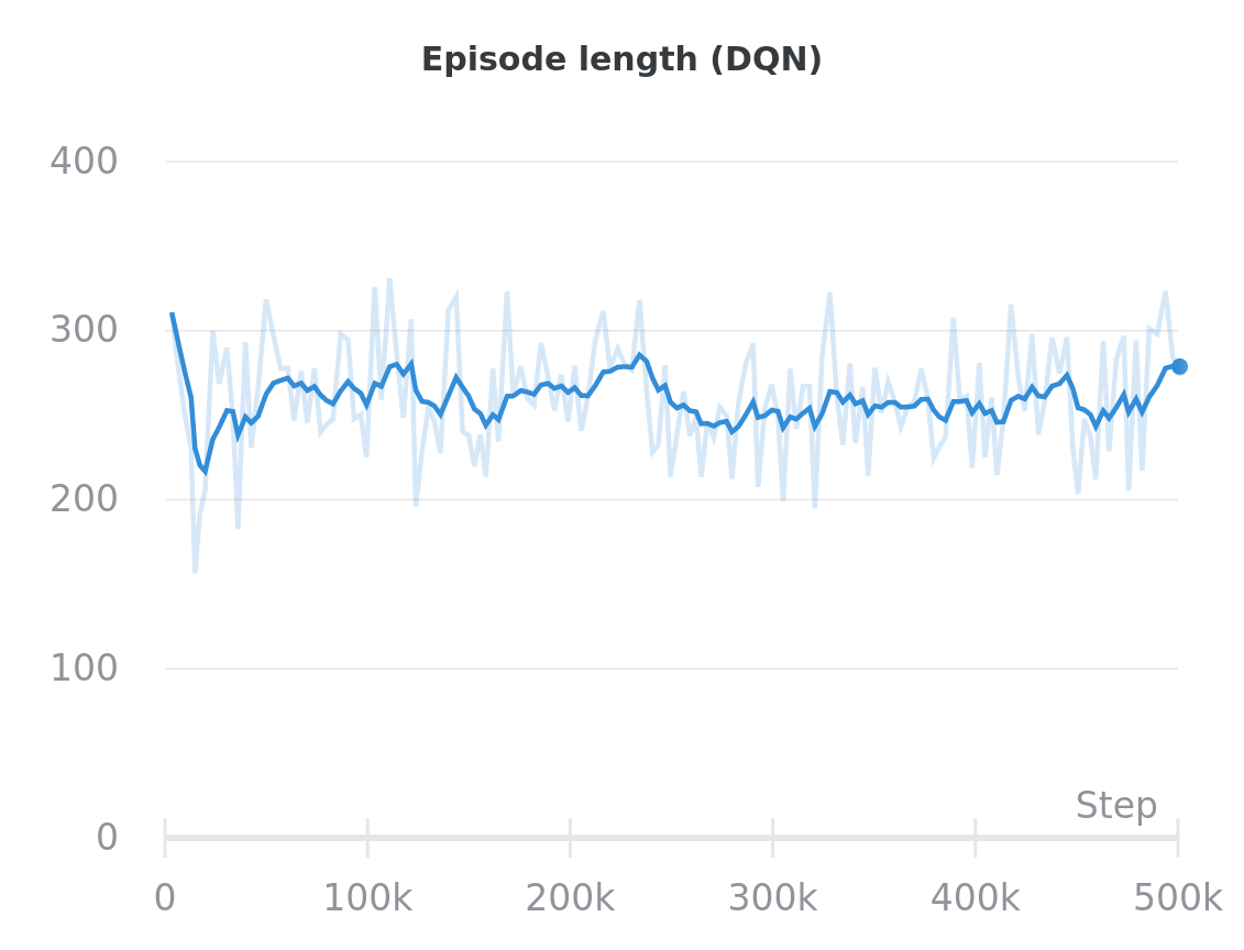
DRQN takes much longer than DQN to converge. The final performance (measured by episode length) of the DRQN agent is a bit better and more consistent, since it is able to systematically explore the environment and avoid revisiting positions seen earlier in a single episode.
DQN
![]()
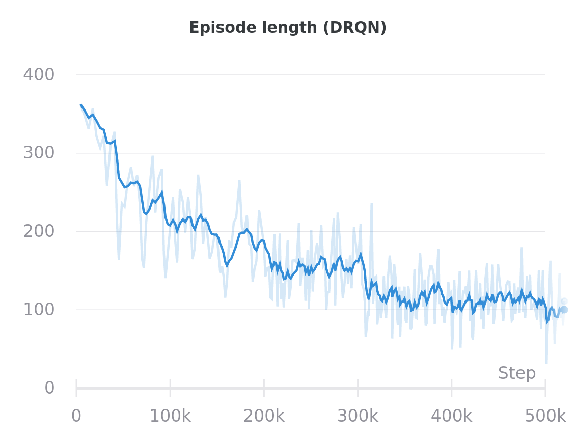
DRQN
![]()
Cluttered environment
Agents in the “cluttered” environments have the same goal as agents in the empty environment, but the environments are filled with static obstacles that are randomly placed each episode. Here the grids are $11\times11$ and have 15 pieces of clutter, and the episode time limit is 400 steps.
The DQN agents are unable to make much headway in this environment; they are only able to attain the goal if they spawn right next to it. The DRQN agents learn to explore the environment and more consistently navigate to the goal square.
DQN
DRQN
References
Matthew Hausknecht et al. Deep Recurrent Q-Learning for Partially Observable MDPs. arXiv preprint arXiv:1507.06527, 2015.
Steven Kapturowski et al. Recurrent experience replay in distributed reinforcement learning. ICLR 2019.
Special thanks to Natasha Jaques for help with this post, and for help improving my DQN/DRQN implementations!