Q learning is a classic and well-studied reinforcement learning (RL) algorithm. Adding neural network Q-functions led to the milestone Deep Q-Network (DQN) algorithm that surpassed human performance on a suite of Atari games (Mnih et al. 2013). DQN is attractive due to its simplicity, but the DQN-based algorithms that are most successful tend to rely on many tweaks and improvements to achieve stability and good performance.

For instance, Deepmind’s 2017 Rainbow algorithm (Hessel et al. 2017) showed that combining double Q learning, prioritized experience replay (PER, Schaul et al. 2015), dueling Q-networks, multi-step learning, and distributional Q learning could outperform standard DQN, A3C, and typically exceed human performance on the benchmark suite of Atari games.

Since the multi-agent experiments I’m interested in don’t really require state-of-the-art performance, and since many of the excellent and feature rich off-the-shelf implementations of RL algorithms do not effectively support multi-agent training, I’ve been implementing the algorithms from scratch. In the interest of managing complexity, I’ve been adding bells and whistles only as necessary.

In a previous post I discussed Deep Recurrent Q-Networks (DRQN), in which agents use recurrent neural networks (RNNs) as a sort of memory that gives them the capacity to learn strategies that explicitly account for past information. This is a key advantage in partially observed environments. As an example, DRQN agents in the exploratory navigation tasks I’ve been studying can learn to use the hidden state to avoid regions they’ve already visited. Learning in partially observed environments is key for MARL, so the scales tipped in favor of implementing DRQN.

I’ve also been using entropy-regularized Q learning with Boltzmann exploration following Haarnoja et al. (2017). I found this strategy for encouraging exploration to be much less finicky than epsilon-greedy exploration.

My DRQN implementation was usually working reasonably well for the environments I’m most interested in (partially observed gridworlds filled with clutter and randomly placed rewards), but training wasn’t quite as stable as I’d hoped. Notably, agent performance would sometimes degrade significantly after long periods of success. Reasoning that the unlearning I observed could be due to catastrophic forgetting once the model began training on only successful episodes, I decided to implement prioritized experience replay.

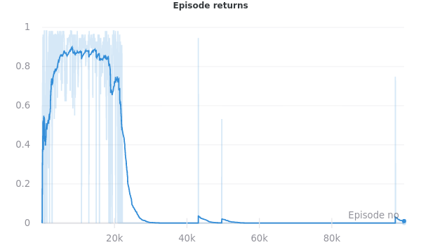
Prioritized Experience Replay (PER) is a key component of many recent off-policy RL algorithms like R2D2 (Kapturowski et al. 2019), and the ablations in the Rainbow paper suggest that PER is among the most important DQN extensions for achieving good performance. Thus I decided to add PER to my DRQN implementation. Sadly PER wasn’t a silver bullet for the particular instability shown above.

Prioritized Experience Replay

Replay buffers and TD errors

In Q learning, agents collect experience following a policy specified by the state-value/Q-function. As the agent interacts with the environment, it periodically updates the parameters of its Q-function to minimize the temporal difference (TD) error of its state-value predictions. As a reminder, the TD error for a transition $(s_{t}, a_{t}, r_{t}, s_{t+1})$ is

and it describes the difference between the agent’s estimate $Q(s_t, a_t)$ of the expected total future return after taking an action $a_t$, and the reward $r_t$ actually observed for that state, plus a discounted bootstrap estimate of the value of the next state $s_{t+1}$.

In tabular Q learning, agents update their Q-functions to reduce the TD error immediately after seeing each transition. Deep Q-Networks (DQN) are far more expressive than tabular Q-functions, but training them in typical deep learning style with stochastic gradient descent (SGD) only works well when they can use batches of uncorrelated samples. Thus DQN agents use replay buffers to store large amounts of past experience. Parameter updates still occur between environment steps but rather than learning from experience as it is collected (as in tabular Q learning), agents sample a batch of data (uniformly) from the replay buffer, then use SGD to update their parameters, minimizing the average TD error on the batch.

1. Uniformly sample a batch of transitions $D_{\text{batch}}$ from the replay buffer $D$,
2. Update the Q-function parameters $\theta$ to minimize the average TD error $\delta_{\theta}$ for $D_{\text{batch}}$ with one step of gradient descent:

Large replay buffers can be helpful because uniform samples are unlikely to be uncorrelated: sampled transitions are likely to come from different episodes, and plausibly include a wider variety of environment states. This helps stabilize training. But larger replay buffers can also lead to slower learning: older experience will have been collected with older versions of an agent’s policy, and thus may not be super helpful for improving the current policy. And of course storing lots of experience requires lots of memory.

Prioritized Experience Replay

The goal of PER is for agents to learn from the portions of past experience that give rise to the largest performance improvement (Schaul et al. 2015). In standard deep Q learning, agents estimate the Q-function’s TD error by sampling transitions uniformly from their replay buffers. With PER, they favorably sample transitions from the replay buffer that have high temporal difference (TD) error. I’ve been using proportional PER, where the probability $p_{t}$ that a sample $(s_t, a_t, r_t, s_{t+1})$ is included in a batch is proportional to the TD error: $p_{t} \propto \delta_{\theta}(s_t, a_t, r_t, s_{t+1})$.

As an example of where this may be helpful, consider an environment with very sparse rewards. Since the agent sees rewards very rarely, the rewards from almost all transitions in the replay buffer will be zero, and the Q-function could pretty quickly converge to something like $Q^{\text{naive}}(s, a) = 0$. Then for a batch to be useful, it needs to contain a transition with a nonzero reward. These are exactly the transitions for which $Q^{\text{naive}}(s, a)$ has high TD error and would be prioritized by PER.

The most straightforward way to implement PER would be to calculate the TD errors for each transition in the replay buffer prior to each gradient update then to use these errors (or some function of the errors) as weights when sampling from the replay buffer to construct a batch. This would be quite costly.

PER avoids the cost of recalculating TD errors for the whole replay buffer before each parameter update by caching TD errors between parameter updates. This is helpful because individual transitions in the replay buffer are typically sampled for gradient updates many times before getting purged from the buffer. Each time a certain transition is used for a gradient update, the TD error for that transition is stored in the buffer to be used as a sampling priority in the future.

Importance sampling

Since PER changes the sampling weights of the transitions in the replay buffer, the distribution of the transitions comprising $D_{\text{batch}}^{\text{PER}}$ differs from the distribution of transitions in the replay buffer overall. This means the parameter gradients computed from TD errors in $D_{\text{batch}}^{\text{PER}}$ are biased estimates of the “true” gradients, so repeated SGD updates might not yield parameters that minimize the average TD error for the whole replay buffer.

This bias can be corrected with a technique called importance sampling, using a weighted average of the sampled TD errors to compute the loss for each batch. The weights are set to cancel out variations in the probabilities that each transition would have been included in the batch in the first place: $w_{i}^{\text{is}} \propto 1/p_{i}$ for the $i$-th sample in the batch¹.

With the importance sampling correction, the procedure for updating the Q-function parameters becomes

1. Sample a batch of transitions $D^{\text{PER}}_{\text{batch}}$ from the replay buffer $D$, weighting each transition by the previous TD error.

2. Update the Q-function parameters $\theta$ to minimize the average weighted TD error $\delta_{\theta}$ for $D^{\text{PER}}_{\text{batch}}$ with one step of gradient descent:

   \[\theta \leftarrow \theta - \alpha \cdot \left( \underset{(s_t, a_t, r_t, s_{t+1}, w^{\text{is}}_{t}) \sim D_{\text{batch}}^{\text{PER}}}{\mathop{\mathbb{E}}} \Big[ \nabla_{\theta} \left( w^{\text{is}}_{t} \cdot \delta_{\theta} (s_t, a_t, r_t, s_{t+1}) \right) \Big] \right)\]
3. Update the TD errors stored in the replay buffer.

Handling recurrence

To train the recurrent Q-function with backpropagation through time, the batches of sampled experience consist of trajectories (of length $k$ « episode length) rather than individual transitions. In order to use PER for trajectory sampling, we need some way to aggregate the TD errors (which are defined for each individual transition) to obtain sequence sampling priorities. I did this by just taking the average TD error for each window, so the sampling probability for the trajectory beginning at $t$ is $p_t \propto 1/k \sum_{i=t}^{t+k-1} \delta_{\theta}(s_i, a_i, r_i, s_{i+1})$.

And to avoid computing this before constructing each batch, I cached these values in the replay buffers alongside the TD errors for each transition, and updated them any time the TD errors changed.

But did PER solve the unlearning problem?

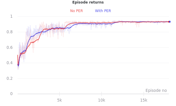
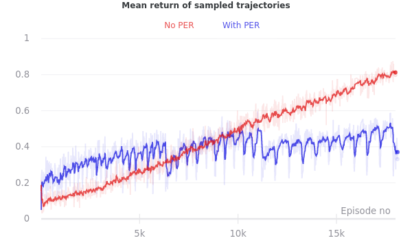
I implemented PER over the course of a few days, after replicating the forgetting described above in a few different environment configurations and hyperparameter combinations. After adding PER, I found that the issue was largely gone! But the impact of PER appeared much smaller when I ran some experiments to measure its impact in a more controlled and rigorous manner.

As it happens, I got better at tuning the other hyperparameters while I was working on the PER code. The improvement to the forgetting issue that I noticed after implementing PER was due in a large part to training with better values of the Q-function’s entropy regularization parameter. PER was helpful (particularly for speeding up training), but for the small partially observed gridworlds with which I’ve been experimenting, I didn’t find (environment, hyperparameter) configurations in which it was decisively important.

References

Volodymyr Mnih et al. Playing Atari with Deep Reinforcement Learning. arXiv preprint arXiv:1312.5602, 2013.

Matteo Hessel et al. Rainbow: Combining Improvements in Deep Reinforcement Learning. arXiv preprint arXiv:1710.02298, 2017.

Tom Schaul et al. Prioritized Experience Replay. arXiv preprint arXiv:1511.05952, 2015.

Tuomas Haarnoja et al. Reinforcement Learning with Deep Energy-Based Policies. arXiv preprint arXiv:1702.08165, 2017.

Steven Kapturowski et al. Recurrent experience replay in distributed reinforcement learning. ICLR 2019.